Localization using encoders
In 2011, the FRC Logomotion had perhaps the best autonomous that highlights a challenge simple enough to make use of encoders to run a predefined distance straight. This article will cover the localization concept, and relate it to predicting physical representation by use of encoders. To start we'll give a general overview of some concepts.
- Laying out a 2D simulated world
- Localization: Using sensors to localize where you are in that world
- trapezoidal motion profiling: considerations for physical motion
- Bench test vs. Actual motion
- Tuning the drive, before encoders (Open loop)
- Understanding motors
- Choosing readable units, factoring gear ratios
- Get real world measurements (top speed)
- Ensure encoder integrity
- Tuning the drive, with encoders (Closed loop)
- Before PID, use assistance for latency considerations
- Using PID
- Putting it all together for actual distance test
Laying out a 2D simulated world
One thing to establish is that we have some coordinate system in a 2D world. This can be represented by X and Y variables and the units can be any unit of measurement. I use meters because it is easy to debug the math with the metric system, and then for any UI I translate them to any preferred units (e.g. feet) as needed. We could use this same technique for a 3D world, but given the nature of the drive, even when going over barriers like in FRC 2016 StrongHold game. 2D can work fine and we would use other sensors to help overcome issues that would alter the 2D location. These variables can be simulated, and later provide real-time updates from the localization techniques.
Localization: Using sensors to localize where you are in that world
When talking about localization it is the techniques used to determine where you are, much like the methods used for gps. The methods themselves are not necessarily set in stone, but are open to add newer methods and combinations of various methods. For us the methods in this case are encoders, but can also include things like accelerometer, gyro, and vision. In this article we'll focus solely on encoders as the sensor, and not cover how to manage multiple sensors, but to be aware that you can. One other concept to add is the idea of prediction, where you lay out a model of where something is predicted to be, and compare against where it actually is, and the difference is the error which can be factored in to the next prediction. One example of this is the GPS. If you are driving a route, the gps can track where you are on that route, but if you deviate from the route and error will kick in to re-route the gps.
trapezoidal motion profiling: considerations for physical motion
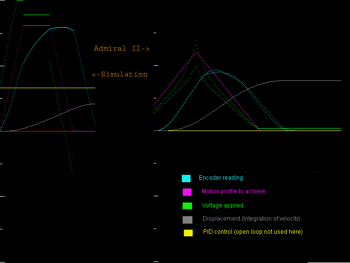
When predicting where something should be, it should take into account the laws of motion. Trapezoidal motion profiling is the idea where a mass ramps up to the "cruising speed" and then ramps down to a stop. When plotting something like this on a velocity graph it looks much like the shape of a trapezoid (See fig 1).

In reality, the transition between ramping to the cruising speed is a smooth rounded corner, but overall still represents this shape. When we put a mass in motion we need to ensure the rate of acceleration is possible by checking the torque requirements, as well as the traction. The JVN calculators help with both of these things. So these set the upper limit of acceleration and deceleration; however, you can go slower than these rates for other considerations.
Bench test vs. Actual motion
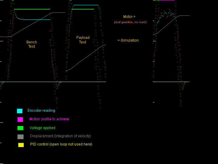
When calibrating the controls it is possible to gather a good estimate from a bench test. This is where the wheels are off the ground and you can test the feedback (See fig 2).

This is often necessary in FRC when working in the pits if calibration is quickly needed. Bench tests do not take on the full load. So for example the highest speed wheels can spin on the bench is around 85% where as with the full load may be 81% of the free load speed of the motor (see motors for more explanation). Luckily for lighter masses you may be able to get away with bench test calibration and the encoders can absorb the error of the full load.
Tuning the drive, before encoders (Open loop)
This next section has taken a long time for me to get right, so I'm going to try to give some detail, because the PID is not necessarily a magic pill that fixes everything. The more error you can avoid, the easier it will be to tune the PID in fact I've been able to keep a generic PID setting for the majority of rotary systems I've tested. So the idea is to model a motion, a ramp up time, a cruising speed time, and a deceleration time, and apply voltage to the motor that will closely fit the trapezoidal model. When doing this there are some guidelines to help make this process a bit easier.
Understanding motors
When using motors it starts by looking at the motor specifications where they call it the motor curve. They produce a graph that shows how fast a motor turns given full voltage and given a variable load. From this, you can predict the motor speed by computing the torque load on the motor, and this graph is linearly scalable so 50% voltage would give 50% of a given speed from a 50% of a given load. The same graph also plots the current but we will not cover that in this article. Perhaps the most surprising outcome from learning this is how it takes time for the actual voltage setting to reach a "steady state" that represents that level, and it may not reach that level depending on the load applied. Finally the moment of inertia of moving a heavy mass influences the load applied so that has to be taken into consideration. When setting motor to a voltage of zero, if the victors are set to coast, the robot will resolve it's own momentum by mechanical friction, otherwise it would keep going (this is more so for a direct drive motor, a motor behind a gearbox may have gearing mechanical advantage to mitigate some backlash).
Choosing readable units, factoring gear ratios
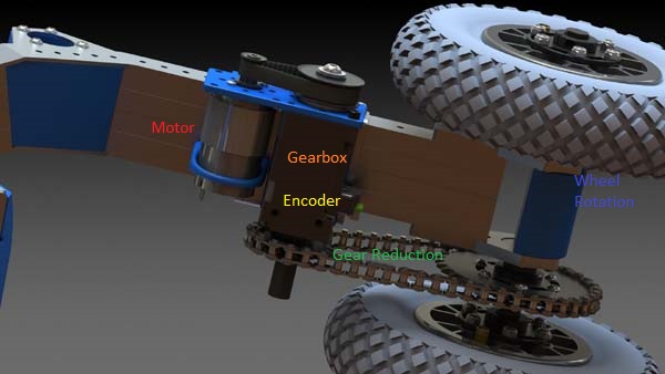
One of the problems I had was trying to figure out the units of what I wanted to track. So for rotary systems that are velocity controlled, I used radians to measure the velocity, but I also have used distance. I've come to the realization that the units I pick are the ones easiest observed. So if I control a drive and wish to control its distance, it is easiest to use units of distance traveled as this is easy to observe. That said, using encoders always measures velocity, but don't let that be the determining factor of what units to use. Instead convert the rate into a more readable unit of measurement and work with that. Note the drive chain...
Voltage->motor->gear reduction->encoder->gear reduction->wheel rotation->distance:

The units observed can be anywhere in this chain. When converting between rotational velocity and linear velocity this is as easy as multiplying the rotations per second by pi D (D is diameter). If using diameter in inches this give the total distance traveled in inches, and since it's rotations per second, it becomes distance traveled in inches per second, where each rotation is transformed to the circumference of the wheel's perimeter.
Get real world measurements (top speed) -Ensure encoder integrity
One problem I faced recently is that the numbers were not adding up properly in my tests, so I wasn't sure if my settings were at fault, or if the encoder was incorrect in its cpr (pulse count). One way to remedy this is to get a video capture of the wheel in full speed motion. When doing this put something on the wheel (e.g. masking tape) to observe as the wheel is spinning around. Capture this on video and preview the frames, given a video usually captures at 30 frames per second (60 is also common), you can easily determine the velocity, with a good accuracy. What I've found is that encoders are usually reliable, as long as the CPR is properly computed as well as the gear ratios of the rotary system. So there should be a match between the visual rotation test and the encoder reading (See Fig 1).
Tuning the drive, with encoders (Closed loop)
As written before, with most of the error minimized in open loop we can then close the loop by enabling encoder feedback.
Before PID, use assistance for latency considerations
Before closing the loop there is one last gain assistance we can do to help minimize error. The way this works is to observe the previous velocity reading to determine if we are accelerating or decelerating by looking at direction of the velocity and then the magnitude between the speeds. From this scale it down to some constant reduction (solved empirically) and add this to the existing voltage. What this does is offers extra voltage during the motion changes. Which minimizes latency because it knows to add more voltage up front to account for the acceleration or deceleration. There is still latency (probably around 90ms) but it will help improve it.
Using PID
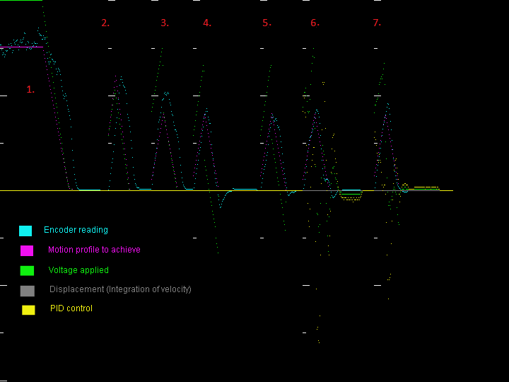
Refer to the following diagram:

In this we have the following:
- Steady state full voltage test to determine max speed
- After speed determined use no gain assist to gather a baseline (notice the latency)
- Try and initial assistance; this shows it being too strong
- This shows a good acceleration, but deceleration may be undesirable
- With deceleration dialed to a likable value, open loop is completed
- This shows closed loop with a P of 200 (I=0 D=25) this looks too powerful to stop correctly
- This is a 100 strength the stopping looks great!
There isn't necessarily a one-size fits all way to tune the PID and many people have their own variation on what they do, but what I show here is what works for me. You may think that open loop 5 looks just as good as closed loop 7, but keep in mind we are on a bench, so yeah on a bench they are equal. Where closed loop shines is when it really is driving to handle the other forces at play, some anticipated like pulling the payload, and some not... possible obstacles and barriers or, perhaps the wheel CoF starts to skid on a slippery surface, or being hit by another robot or game piece etc. Note: that I put the P at 100 for the bench, but it may turn out that I use 200 for testing the real driving. We give it the best bench tests, and keep actual drive tests to a minimum as it may be hard to find time for them.
Putting it all together for actual distance test
As a simple test, it is much like the bench test I test to drive for 2 feet forwards and then backwards. I look the number of rotations the wheel turns. In this test I didn't have the tuning completed yet where it looks like #3 with a P set to 200, and as a result you can see the center wheel start to peel out a little. Ideally a test like this would be just like the bench and I can compare the difference. When I test this I don't need to make the graphs like I'm showing here, I can get a good idea just from reading the raw dump to save time. I did automate a way to present live graphs, but found I kept forgetting how to set that up, so I just use pure text dumps and this works fine. It should be noted the test itself sets a way point with a loose tolerance, so while I test for 2 feet, the actual way point code may have a loose tolerance to stop short. When doing a navigating type of goal, loose tolerance is fine as there are continuous corrections taking place, but that does not matter for this test. What matters is that whatever the distance it told the robot to move, that it can handle that as well as possible. As long as the raw dump shows the correct numbers... that is where to verify first... and test for consistency. When I did the test above, I ran two forward tests, and two back tests all 2 feet. It was consistent and put the robot back to where it started. There may be external errors, so if the rotations add up properly, the error may be in the actual circumference in the wheel, but if it's consistent it may be possible to account for these errors, or leave it be and find some way to continue to make corrections, such as vision.
